Embeddings and its applications

With the popularization of tools boosted by Large Language Models, such as ChatGPT from OpenAI, LLama3 from Meta, or Claude 3.5 from Antrhopic, the "embedding" word became known and popular by people who do not have a background in Natural Language Processing related fields.

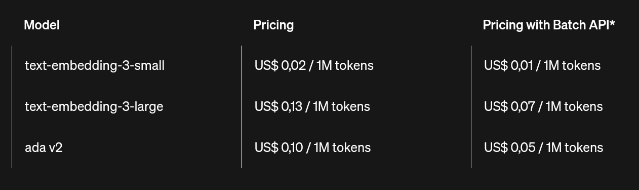
If you already visited the OpenAI API pricing page, you probably noted the models text-embedding-3-small, text-embedding-3-large, and ada-v2, cost way less than the well known LLM models as gpt-3.5-turbo or gpt-4o.

In this post, we are going to understand what Embeddings are, their functionalities, and understand their relevance in LLM applications, like semantic search and text clustering.

The Embeddings

The process of transforming text into embeddings involves converting text (as readable by humans) into a vector representation (here denominated by V), that belongs to a vector space R with n dimensions (R^n).

For each phrase (or text) there will be a vector, allowing us to make comparison between vectors from the same vector space, e.g., by calculating the angle and distance among all vectors of that space.

In simple terms, embedding transformation is how we translate human language into something that computers can understand, allowing us to compare different phrases (now as vectors) and group the ones with some similarity.

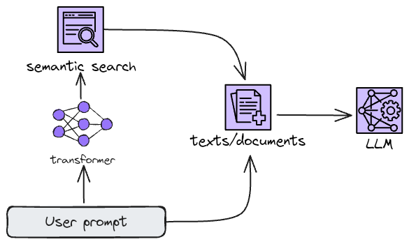
This transformation, combined with a vector database, allows the so called semantic search, allowing you to provide context to your preferred LLM. This technique is known as RAG (Retrieval-Augmented Generation), and in my opinion, it is one of the best ways to use a LLM nowadays. I will not get into details about RAG in this post, but I highly recommend you research this field and explore its potential (after you finish reading this post, of course!).

To conclude this section, remember that embedding transformation does not resume the numerical transformation of texts; it is also possible to get embeddings from other kinds of data, like images and audio.

Background

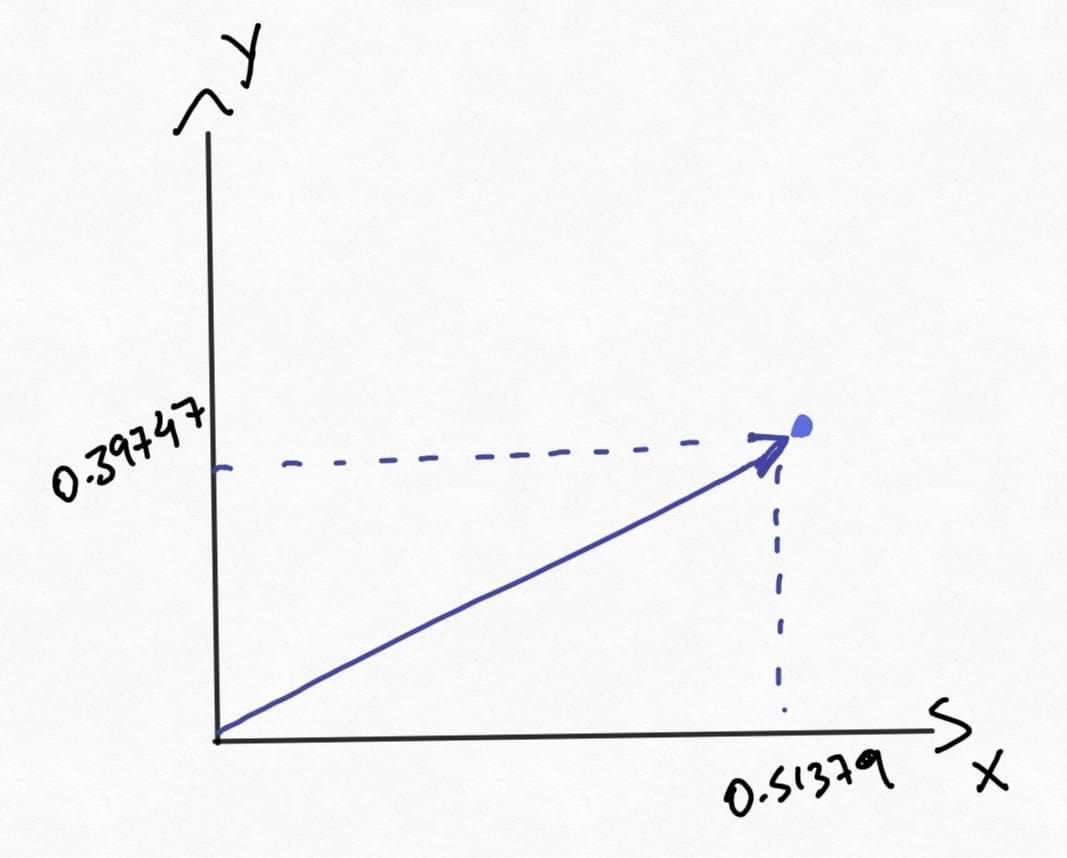
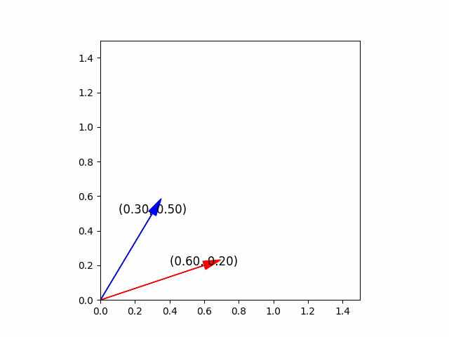
For those who have never seen linear algebra before, let's start with a simple 2-dimensional vector. In this post, the 2D vector space (here called R2) will be represented by the x-y plane, where a point in this space is defined by two coordinates (x, y). In the image below we define the vector V1 (in purple) at the coordinates (0.51379, 0.39747).

Therefore, let's define a vector space as the space where we can perform an addition operation between two vectors, and/or multiply them by scalars, e.g., we can take vectors V1 e V2 and multiply them by a scalar of 2, increasing their magnitudes twice inside the vector space, while preserving their directions. These properties - addition and multiplication - are valid for all vectors within vector space.

At R2 space, or even at R3, it is easy to imagine the vectors. Now, imagine (or at least, try) a vector in a vector space of 5, 8, 13, 21, or 1232 dimensions! It is completely out of our capacity to render it mentally.

With the main concepts set, we can start to explore the concept of similarity search, i.e., to verify if two or more vectors are pointing in the same direction and/or if they have similar magnitudes.

It is important to note, that there are different methods to check for similarity between vectors, where the two most popular are the Euclidian distance among the coordinates of the vectors; and the similarity by the cosine between two vectors.

Since I use the cosine method at the most to perform similarity search, I'll use this method to continue the explanation.

The cosine similarity is given by the equation below:

$$ cos(\theta) = \frac{V_{1} \cdot V_{2}}{\left| V_1 \right | \left | V_{2} \right|} $$

What we are doing is to calculate the internal product between the two vectors and divide the result by the product of the module of each vector. In that way, we can obtain the cosine similarity between them.

If studying linear algebra is not possible for now, it's enough to know that if the result from the calculation above is equal to 1, then the vectors are pointing in the same direction, and if the result is -1, they are exactly in opposite directions.

As an example let's calculate the similarity between V1 and V2.

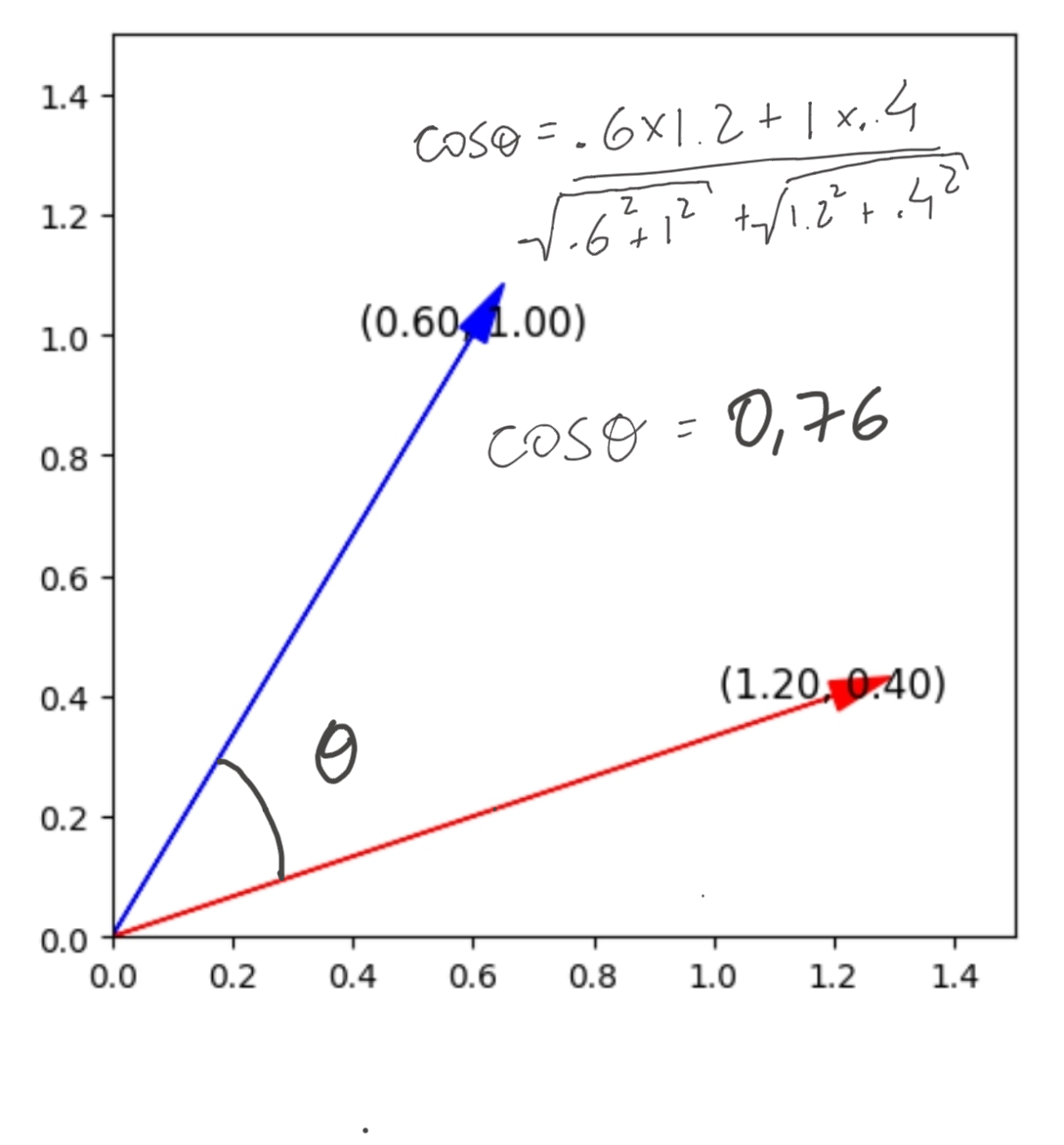
From above, we can conclude that the vectors V1 and V2 have a similarity of 76%.

Connecting the dots

Now that we acquired a small understanding of vector space, vectors, and similarity among vectors, it is easier to integrate everything with what was explained about embeddings at the beginning of this post.

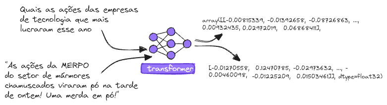
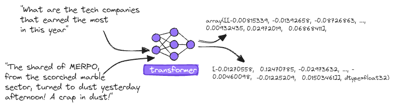
Embeddings, as said before, are representations of things as vectors, in the case of this post, it always will be text data. Therefore, let us take a look at a real example by considering the sentences below and calculating the similarity among the sentences F2 and F3, in relation to F1.

Note: the original post was wrote in portuguese, and so the sentences, therefore, I will just translate them to english and preserve the result.

Note: the last sentence makes more sense in portuguese since MERPO was a joke inside the brazilian stok market.

In the next section, I will show in detail how to obtain the embeddings and the different options to do it. For now, let's only use the model all-MiniLM-L6-v2 and get the embeddings (as vectors) for each sentence above.

sentences = [
    "What are the tech companies that earned the most in this year",
    "Totvs (TOTS3) is one of the tech company that earned the most in this year, reporting several millions Reais in profit in the latest quarter.",
    "The shared of MERPO, from the scorched marble sector, turned to dusty yesterday afternoon! A crap in dust!"
]

from sentence_transformers import SentenceTransformer

model = SentenceTransformer("all-MiniLM-L6-v2")
model.max_seq_length = 256

embeddings = model.encode(sentences, normalize_embeddings=True)

display(embeddings)
display(embeddings.shape)

As output we have 3 vectors... but with way more than 2 coordinates for each vector! As I said before, a vector space can have more dimensions than our brain can render geometrically.

In the case of all-MinilM-L6-v2 each embedding has 385 dimensions! (and this is small when compared with other models)

array([[-0.00815339, -0.01392658, -0.08726863, ...,  0.00932435,
         0.08745421, -0.01407533],
       [-0.02574616, -0.02340927, -0.09131505, ...,  0.01132488,
         0.02972019,  0.06868411],
       [-0.01270558,  0.12470785, -0.02973632, ..., -0.00460098,
        -0.01225209,  0.01503461]], dtype=float32)
(3, 384)

Now we can verify what is the similarity between F2 and F3 in relation to F1 by computing the cosine among the vectors. Obviously, I will not compute it by hand and I will use the cosine_similarity method from sklearn package in a small Python script.

from sklearn.metrics.pairwise import cosine_similarity

v1 = embeddings[0].reshape(1,-1)

for i in range(0,3):
    cos_sim = cosine_similarity(v1, embeddings[i].reshape(1,-1))
    print(f"Similaridade entre F1 com F{i+1}: {cos_sim[0][0]}")

Similarity between F1 and F1: 1.0
Similarity between F1 and F2: 0.6518208384513855
Similarity between F1 and F3: 0.3244129419326782

And as we were expecting, the F2 sentence has a higher similarity with F1 sentence, not only by the similar words, but by its overall context!

The real power of the embeddings is the capacity to transform chunks with meaning into vectors.

How to get the Embeddings

The mathematical representation of texts is not a new concept and can be achieved using simpler models, such as the Bag of Words (BoW). In this approach, the frequency of words within a sentence or document is counted. This type of model is very efficient for tasks involving text classification.

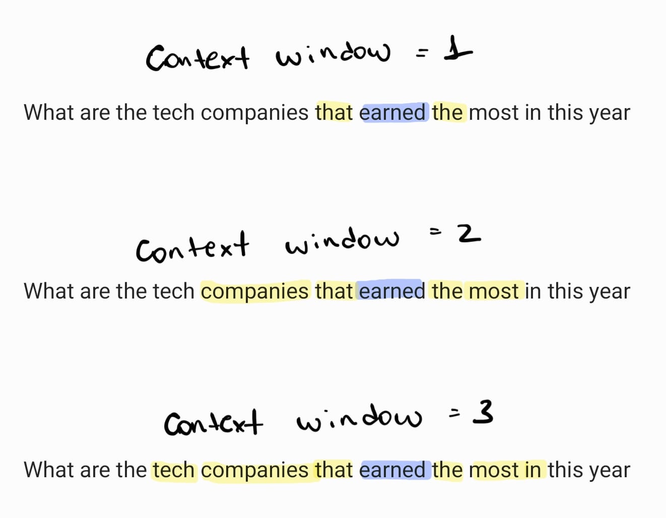
With the application's increase of Recurrent Neural Networks (RNN) to the Natural language Processing (NLP) field, in particularly with google contributions with the model Word2Vec in 2013, the process to obtain embeddings now takes into account the surrounds of the words, i.e., a context window.

But what allowed big changes in the NLP field and set the stage to use Large Language Models (like chat-gpt, gemini, etc) as we use today, was the introduction of a new neural network architecture, denominated as Transformer. (Vaswani et al., 2017)

Delving deeper into the explanation of the transformer architecture would require a separate post. For now, it is enough to know that the core of the transformer system enables longer sentences to be processed more efficiently and with less computational power compared to models like Word2Vec.

The embeddings generated as examples in the last sections were obtained by the Python package SentenceTransformer, well known as SBERT.

Besides the SBERT, I frequently use the model text-embedding-3-small from OpenAI API, with 1536 dimensions for each vector. In one of the semantic search projects that I worked with, I obtained better results with it compared to SBERT.

The downside is the need to set up a paid account and fund it before using the API. We pay per quantity of token to be transformed into embeddings. But to be honest, the cost is really small and the better results justify the use in most cases.

Applications

This post explained semantic search, where we search for similar meanings in texts or documents. But there is another special application, which also uses the semantic search power, named RAG.

RAG stands for Retrieval Augumenthed Generation, and this technique is nothing more than providing context directly in the prompt before the LLM processing.

In this way, the LLM uses the provided context to answer the user, allowing to creation of systems where the context can be retrieved as new and updated data.

If playing with the semantic search is all that you want to do, the Python script above is a good starting point, and the SentenceTransformer package itself has a method to compute the similarity between vectors.

But if you want to go deeper, we begin to deal with vector databases, such as Qdrant, which is designed to store embeddings and enable efficient searches within it.

Soon I will be posting here an article where I go through all the processes, starting from the embedding obtaining, and storage, and finishing with LLM integrations.

Text Clusterization

Text clusterization is another application where embeddings are key.

To cluster texts, we make use of unsupervised clustering algorithms, where the most famous is the K-means model.

I will not go deep in the mathematical formulation of the k-means, just know that this model uses the distance between two points to determine if those points are similar or not. And since the embeddings are nothing more than points in a vector space, it is clear that we can apply the K-means algorithm to tell if texts (as embeddings) are close enough to each other to make groups.

But hold on! We can't just pick all vectors, with 1534 dimensions each, and apply k-means and get good results. Unfortunately, there is a phenomenon in the data analysis known as the "curse of dimensionality", where, as the number of dimensions increases, the meaning between two data points decreases, since all distances become too similar to each other.

To avoid the curse of dimensionality we can apply dimension reduction techniques, where we can reduce 1534 dimensions to only 3 dimensions.

Among the dimension reduction techniques, we can name a few like the t-SNE and UMAP, but since this post already got too long to read, I will let this clusterization topic into another post.

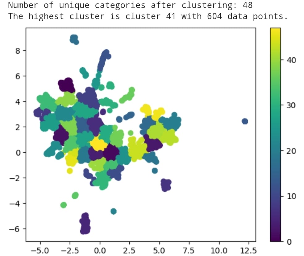
To close this topic, below is the result of a clusterization of more than 12 thousands descriptions of AI tools that I performed aiming to classify the tools into common categories. The result was quite good, with 66 classified categories.

Conclusion

I hope my goal of explaining what embeddings are and how to apply them was reached.

If this text was helpful to you, share it with anyone who might benefit from it as well. If you have any questions, feel free to connect with me on LinkedIn and we can discuss further.

References

1. Pilehvar M.T., Collados J.C. - Embeddings in Natural Language Processing - Theory and Advances in Vector Representation of Meaning (2020).
2. Gilbert Strang - Linear Algebra and Its Applications (4ed)-Brooks Cole (2005).